Understanding Gradient Boosting as a gradient descent

There are a lot of resources online about gradient boosting, but not many of them explain how gradient boosting relates to gradient descent. This post is an attempt to explain gradient boosting as a (kinda weird) gradient descent.

I’ll assume zero previous knowledge of gradient boosting here, but this post requires a minimal working knowledge of gradient descent.

Let’s get started!

For a given sample $\mathbf{x}_i$, a gradient boosting regressor yields predictions with the following form:

where each $h_m$ is an instance of a base estimator (often called weak learner, since it usually does not need to be extremely accurate). Since the base estimator is almost always a decision tree, I’ll abusively use the term GBDT (Gradient Boosting Decision Trees) to refer to gradient boosting in general.

Each of the base estimators $h_m$ isn’t trying to predict the target $y_i$. Instead, the base estimators are trying to predict gradients. This sum $\sum_{m = 1}^{\text{n_iter}} h_m(\mathbf{x}_i)$ is actually performing a gradient descent.

Specifically, it’s a gradient descent in a functional space. This is in contrast to what we’re used to in many other machine learning algorithms (e.g. neural networks or linear regression), where gradient descent is instead performed in the parameter space. Let’s review that briefly.

Gradient descent in parameter space: linear regression

We’ll briefly describe a typical least squares linear regression estimator, optimized with gradient descent.

Let’s consider the least squares loss \(\mathcal{L} = \sum_i (y_i - \hat{y}_i)^2 = \sum_i (y_i - \mathbf{x}_i^T\mathbf{\theta})^2\), where the predictions $\hat{y}_i$ are defined as:

In order to optimize the loss with respect to $\mathbf{\theta}$, a gradient descent consists in starting with a random $\mathbf{\theta}$ and iteratively updating it¹:

In code:

theta = np.zeros(shape=n_features)  # or some actual random init
for m in range(n_iterations):  # or until another convergence criterion
    negative_gradient = -compute_gradient_of_loss(y, X, theta)
    theta += learning_rate * negative_gradient

There are a few important things to note:

• The optimal $\mathbf{\theta}$ that we end-up with can be expressed as a sum: $\mathbf{\theta} = \sum_{m=1}^{\text{n_iter}} b_m$, where the $b_m$ are the product of the learning rate and the negative gradient. Notice how similar this sum is to what a GBDT predicts.
• In this case, we compute the gradient of the loss with respect to the parameter $\mathbf{\theta}$. In gradient boosting, we compute the gradient of the loss with respect to the predictions $\hat{y}_i$.

Wait, what?

Computing the gradient of the loss with respect to the predictions $\hat{y}_i$ is something that I found quite confusing at first, but it actually makes a lot of sense. Consider the following:

The general purpose of gradient descent is to minimize a function, with respect to one of its parameters (any parameter, BTW).

In linear regression, the function that we minimize is the loss $\mathcal{L}$, and the parameter that we choose is $\mathbf{\theta}$.

But the predictions $\hat{y}_i$ are also a parameter of this loss function: remember the definition $\mathcal{L} = \sum_i (y_i - \hat{y}_i)^2$!

These predictions $\hat{\mathbf{y}} = (\hat{y_1}, \cdots, \hat{y_n})^T$ are actually just a vector in $\mathcal{R}^n$, just like $\mathbf{\theta}$ is a vector in $\mathcal{R}^d$.

So, conceptually, there is nothing keeping us from minimizing the loss with respect to the predictions.

Let’s try that.

Minimizing the loss with respect to the predictions

Just like we started with a random $\mathbf{\theta}$ before, we’ll now start with random predictions. The update rule becomes², for all training samples $i$:

We literally just replaced $\mathbf{\theta}$ by the $\hat{y_i}$ here. Taking the least squares loss again, we have:

Now, let’s actually code this gradient descent, and verify that the loss is indeed minimized. There’s a bit of boilerplate but the code is deceptively simple.

from sklearn.datasets import make_regression
import numpy as np
import matplotlib.pyplot as plt


def least_squares_loss(y_true, y_pred):
    return np.mean((y_true - y_pred)**2)

def compute_gradient_of_loss(y_true, y_pred):
    # Gradient of LS loss w.r.t y_pred
    return -2 * (y_true - y_pred)

n_features = 10
n_samples = 1000
n_iterations = 30
learning_rate = .05

X_train, y_true_train = make_regression(n_samples=n_samples, n_features=n_features)
y_pred_train = np.zeros(shape=n_samples)
loss_values = []

# Gradient descent on the predictions. Note how similar that is to the
# gradient descent on theta above.
for m in range(n_iterations):
    negative_gradient = -compute_gradient_of_loss(y_true_train, y_pred_train)
    y_pred_train += learning_rate * negative_gradient
    # save loss value for plotting
    loss_values.append(least_squares_loss(y_true_train, y_pred_train))

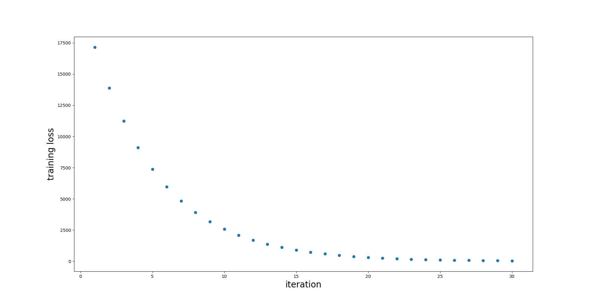
plt.plot(np.arange(n_iterations) + 1, loss_values, 'o')
plt.xlabel('iteration', fontsize=20)
plt.ylabel('training loss', fontsize=20)
plt.show()

Gradient Boosting: use the base estimator to predict the gradients

Looks like it works! The loss decreases and is very close to 0 after a few iterations. That means that we are able to predict the values in the training set with almost perfect accuracy.

Of course, this is pretty much useless in practice :)

Ultimately, what we want to do is predict values for unseen samples, not for our training samples. With the code snippet from above, we have no way of predicting for unseen values.

But there’s a pretty simple trick that will solve this issue: instead of updating $\hat{\mathbf{y}}$ with the real value of the gradient, we will let a base estimator predict these gradients, at each iteration. This set of base estimators are able to output a prediction for any sample, not just the samples in the training set!

We go from:

# previous version, as in code snippet above
for m in range(n_iterations):
    negative_gradient = -compute_gradient_of_loss(y_true_train, y_pred_train)
    y_pred_train += learning_rate * negative_gradient

to

# Gradient boosting, letting a base estimator predict the gradient descent step
predictors = []
for m in range(n_iterations):
    negative_gradient = -compute_gradient_of_loss(y_true_train, y_pred_train)
    base_estimator = DecisionTreeRegressor().fit(X_train, y=learning_rate * negative_gradients)
    y_pred_train += base_estimator.predict(X_train)
    predictors.append(base_estimator)  # save predictors for later

We can now output predictions values for any samples by summing over all predictors:

def predict(X):
    n_samples = X.shape[0]
    predictions = np.zeros(shape=n_samples)

    for h_m in predictors:
        predictions += h_m.predict(X)

    return predictions

Well, this predict function is just another way of writing our initial formula:

And that’s our gradient descent in a functional space.

Instead of using gradient descent to estimate a parameter (a vector in a finite-dimensional space), we used gradient descent to estimate a function: a vector in an infinite dimensional space.

Wrapping up

There are 2 main things going on:

1. Instead of taking the derivative of the loss with respect to the parameter of a parametrized model, we take the derivative of the loss with respect to the predictions. There is no notion of parametrized model anymore, but we’re still able to minimize our loss on the training samples!
2. At each iteration of the gradient boosting procedure, we train a base estimator to predict the gradient descent step. Saving these base estimators in memory is what enables us to output predictions for any future sample.

If you want to have fun, I made a notebook with a pretty simple implementation of GBDTs for regression and classification.

I hope you now understand why Gradient Boosting can be considered as some form of gradient descent.

I would greatly appreciate any feedback you may have!

For a follow-up on how GBDTs for classification work, and other details, check out this follow-up post.

Resources

There is much more to gradient boosting than what I just presented!

I strongly recommend this tutorial by Terence Parr and Jeremy Howard. They also have a nice section about gradient descent.

The initial gradient boosting paper Greedy Function Approximation: A Gradient Boosting Machine (pdf link) by Jerome Friedman is of course a reference. It’s quite heavy on math, but I hope this post will help you get through it.

The Elements of Statistical Learning by Hastie, Tibshirani and Friedman, also have a nice coverage of gradient boosting (on the mathy side too).

Nicolas Hug

ML Engineer

Tweet Share